The Fierce Urgency Of Now
The Fierce Urgency Of Now:
“You have to let ideas win,
not hierarchy.” – Steve Jobs.
Mark Suppes is out. The
community is devastated to see him go.
Why did this happen? Money - Mark
needed support, and he never got it.
This has become very common; even for the best researchers. Dr. Klein had an Ivy League PhD, publications
and experience from Oxford [47]. Any
idea from him had been scrutinized. Why
then, did it take him ten long years to get funding?
Money is
always a tough issue. The US spends
about 400 million on fusion a year.
Recently, this money has been changing directions. NIF is declining. Its budget is down 20% for next year. This is probably because the machine failed to
ignite. Next, ITER is rising. It will eat over half the budget. Meanwhile, domestic programs are ending. MIT’s tokamak may fall in October. We are sorry to see them go – but we gave
them 41 years, and there are still no tokamak power stations [40, 41].
When a 14 year old kid can fuse atoms in his garage – it screams revolution. It says that fusion energy will have nothing
to do with a big machine in France. The
final solution may not be a polywell.
But the answer lies somewhere down that road. To get there, we need broader funding. Why focus on two well-worn ideas, when
alternatives exist? The ITER machine got
a 75 million increase this year. That
could have funded ten new ideas. If we
stay on this path; we will never get there.
We need to get there. Burning carbon is
killing our world. It causes global
warming. It is unsustainable. We know we need to change. Sustainable energy is only way out. To win, it must scale. To win, it must be cheaper than carbon. Fusion energy could be that solution. Today, we have brand new ways to get there. So, what are we waiting for?
"Vision is the art of seeing what is invisible to others." –Johnathan Swift
Executive
Summary:
This post
reviews work measuring electrons inside a polywell. The Australian team used a new
biased probe to find electron density, temperature, speed and the local
voltage. This data came from reading the
current drawn by the probe. Due to cost
limitations, this analysis could not be automated. Precise equations for the plasma and probe
were fitted to the data, ad hoc. A new
4” aluminum polywell was used. Results
from simulations are also presented. Five
tests were done. First, a beam was
measured, and this bench marked the probe and analysis. Second, the center was checked with and
without a magnetic field. The results supported electron trapping. Next, measurements were made along the x-axis
and this also showed trapping. The
fourth test looked at the effect of the ring field on the electron cloud. Data showed that the potential well rises with ring strength. Finally, the
impact of the electric field on the potential well, was tested. As more and
faster electrons are injected, the center gets more negative. This ends when speedy electrons, start to escape the ring field. The details of the paper are in the appendix,
and select data can be downloaded here.
News:
After an ode
to the fusioneer was posted in April, work focused on the polywell 101. The film explains the machine using a
voiceover and a whiteboard. It addresses:
mechanism, design, operation and challenges.
That work was part of a collaboration, with the folks at Talk-Polywell. Thanks to everyone who helped out. In May, the world passed 400 ppm of carbon
dioxide - a clear sign that we need new energy sources. Also in May, Dr. Joe Khachan published
another paper in physics of plasma. This
post will review that work. That month,
the Turkish atomic authority published a fusor paper. Their machine was about a foot across and
produced 2E4 neutrons per second [44].
This was done with an 85 kilovolts drop across the cages. This implies they used some costly equipment. Those specs put the Turkish team near the
high end of the amateur scale. They have
better equipment; but Richard Hull has gotten more neutrons. Photos of their equipment are shown below.

The Turkish paper mentions polywells and penning traps as
the next step [44]. We cannot know if
they will build one (their vacuum chamber is not appropriate) however, it is a
possibility. Bottom line: we now
have a new group in the game. In August, the Polywell was included in an MIT competition for solutions to the climate crisis. You can vote for it, by logging in here.
“I
hoped that a venture capitalist would get excited and say: Let’s Do This! It never happened.” – Mark Suppes
Review of May 2013 Paper:
Overview:
This goal of
the Khachan work is to prove that electrons are trapped in a Polywell. This has been shown before [17] but we can now
get more details about the electrons.
This paper will measure the electrons density, temperature and speed
inside a polywell. It will also
connect this to the magnetic and electric fields in the machine. This work is exciting, but the results are
limited. The team did not have tons of
cash to work with - and it shows. Their
polywell was small and it had a low power source. Their probes and analysis were homemade. They squeezed as much data out of this setup as
they could – but they will need more funding to go farther. We need to give them that support.
These new details are because of a Langmuir probe.
For ninety years, these probes have been used to measure plasmas [33]. The team is using a brand new biased probe. It is a
thin tungsten wire with a voltage applied to it. This lets them collect new data about the
electrons. This data will be used to build
the case for electron trapping. The team
will argue this case - as if they were lawyers in a courtroom.
Their
argument will be structured around four experiments. The first is a test case. The probe is stuck in the center of a
non-working polywell. It will measure a
beam of electrons as they pass by. This
test will bench mark the probe and analysis.
The second test compares a working and non-working polywell. Predictably, when a magnetic field is added,
it changes everything. The third test moves
the probe around during operations. The
electrons are measured along the x-axis. This will show the environment at
different places inside the cloud. The
fourth test has two parts. First the
voltage drop in the center is monitored while the ring strength changes. Second, the voltage drop is measured while
the electric field changes.
Experimental
Setup:
These new measurements require a new
setup. About half the setup changed from
their 2010 paper. They used the same
vacuum chamber and polywell mount [27, 16, 17].
They powered the rings with the same set of capacitors; although two car
batteries were added on. What are new -
are the probes, injectors and polywell.
Three probes were added. Each
probe was a long, thin wire, with backup equipment. Details on the probe are included below. The team used six light bulb filaments for
injectors. When these wires heat up,
electrons are kicked off. They fly
towards the positive polywell and get trapped.
These injectors make plasma, of a known density. This was vital for data analysis. Lastly, they built a new aluminum
polywell. This setup is pictured below.

A
New Polywell:
Like
their old Teflon polywell - this aluminum device is also about the size of a
coffee cup. We used photos to estimate
the size [23]. The rings were 2.25
inches in diameter. Each ring had a
cross section, a half inch in diameter.
The rings were smooth aluminum shells, with 15 coils of coated copper
wire inside. The smooth surface is
critical for success. The shells were
made by metal spinning [17]. A thin disc
of soft aluminum is centered on a lathe.
The disc is spun at high speeds.
A wedge is pressed into the metal.
As it spins, the metal curves around the wedge [22]. This is an inexpensive way to make the device. A photo is shown below.

Spinning made twenty-four parts that needed to be
assembled to make the Polywell. In the
picture, this is done with metal ties and soldering. During experiments, ties or clamps were used
to hold the rings together [27]. This
was needed because during peak use, each ring was pushed apart with 15 pounds
of magnetomotive force [appendix]. Unfortunately,
the clamps pierce the stream of recirculating electrons. This creates problems [29]. Electrons that touch the clamps could be
lost. Losses are made worse, because the
clamps and the rings were all held at a positive voltage.
Improvements:
How could
we improve this device? First, the
clamps cannot remain. With no clamps,
one must bond the rings together. Unfortunately,
spot and arch welding are both out. They
would melt everything and make a mess of delicate parts. Soldering is preferable. This narrows the options for ring materials. One possibility is 3003 aluminum. This is pliable for spinning and good for
soldering [24, 19]. The metal can be
soldered at 220C [25]. This temperature
will not melt the copper wire inside, but it may burn the wire cladding. To do this, the shells would be heated on a
hot plate and a solder wire would be applied [26]. Afterwards the part may be sanded for a
smooth surface. The final device would be made of aluminum, with traces of tin
and silver. Materials selectors will
also need to consider: neutron activation, thermal conductivity and magnetic
transparency.
Langmuir Probes:
Background:
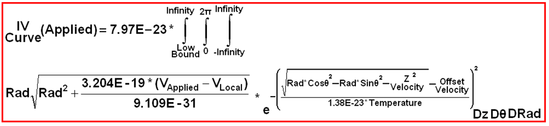
These probes were made by Nobel laureate Irving Langmuir. You stick a thin wire into the cloud. As the positive and negatives touched the metal, a current is drawn from the wire. This is a cylindrical probe [36]. You biased this wire at some voltage. As the wire changes from negative to positive, the current also changes. This signal is known as a current-voltage or IV curve. From this data: the plasma density, energy, charge and potential can be found [37]. But this is not easy. You need to do some mathematic acrobatics to get it to work [34]. Reading this signal is actually its own field of study. Normally, you outsource this work to a company with software and fancy tools [35]. But the team had no money. They had to tackle this analysis by hand. Each wire-plasma interaction was analyzed ad hoc. Here is an illustration of this process.

There are some key facts about this analysis. First,
voltage changes throughout a plasma cloud.
This is called the local voltage. The wire must be stuck in to measure this voltage. The volume around this wire is called a
sheath. This is a plasma filled region. The plasma in the sheath behaves differently than
the rest of the cloud. This behavior
comes in two types. In type one the wire
is positive compared to the cloud. This
means that the wire voltage is greater than the local voltage. Here, electrons
cluster around the wire. They are
attracted to the positive charge. The
sheath is filled with electrons - and all of them touch the wire [42]. In type two, the wire is negative to the
cloud. Here, electrons are
repulsed. Any negative charge that touches
the wire, must have overcome this repulsive field. To do this, they need a minimum
velocity. This velocity can be estimated
and must be included in the analysis. These
two types are illustrated below.

Rules
for Langmuir Probes:

Math
and Data:
Nobel
Prize winner Irving Langmuir worked all these rules
out [42]. He reasoned that if
electrons follow his rules, he could predict the current to the probe. His analysis relied on the plasma velocity
and the type of probe. Using these
conditions, he designed math to go with them.
That is powerful. It means you
can fit equations to data. In doing so -
you can find the local voltage, density and energies. This is what Khachan will do. They will stick wire probes into four
different polywell setups. The probes
will draw current. This data will then be
fitted to specialized equations. Based
on the fit, plasma information will be found.
Fitting requires two expressions.
The first is for the wire and the second is for the plasma. The wire equation is a general cylindrical probe
equation that applies to all wire probes [42].
This expression is shown below.


Plasma
Equations:
The
equation for the plasma is a velocity distribution for the electrons. Working out the velocity distribution is the
hardest part of this paper. It must be
done on a case by case basis. The team has
three velocity distributions to choose from.
The first is for normal electrons with a bell curve of velocities. They never use this - and that is a key
fact. None of the electrons measured
here appear to have bell curves of energy.
The second is for a beam of electrons, all near the same speed. This “beam analysis” is used several
times. The third expression is for
electrons in a cloud, all near the same speed.
The challenge is picking the right expression for the plasma
tested. The velocity and probe equations
are combined and integrated. This leads
to nasty integrals which can only be solved numerically. This work is shown in the appendix. Their solution predicts current to the probe
at a given voltage. When equation and
data are fitted together, measurements pop out.
Test I: A Beam
The team
started with a simple experiment to verify their analysis works. They measured the electrons in a beam. We expect beam electrons to be monoenergetic
[45]. The electrons should all be at the
same temperature and the thermalization ratio should be low. This is a situation where we know what we
should get. If the data matches
prediction, it benchmarks the probes and the analysis.
The
setup they had was simple. They put one
emitter seven centimeters away from polywell center. When electrons were kicked off, they become
attracted to the rings. This is because
the rings are at a positive 150 volts. A
probe is stuck in the center of the Polywell.
This wire will absorb some of the electrons, making an IV curve. The team expects a certain IV curve. An illustration of this is shown below.

Basic models can predict much about this
setup. First, the
electrons are moving along the x-axis.
Along this axis, the polywell is symmetric. Therefore we can ignore four of the
rings. The two remaining rings are treated
like flat discs. These discs are loaded
with positive charge. This charge makes
the rings positive and attracts the beam.
The field made by one ring can be predicted with a simple
equation [38, 39]. The total electric
field is a superposition of two disc and this can predict electron speed. The model is explained in detail in the
appendix. Our model predicts about one
third the measured electron speed near the probe. That is pretty good.
Beam
Velocity Distribution:
Electrons
in a beam can be modeled as having the same energy [43]. But, real life is different. The energy will spread out some. Langmuir developed the original equation [42]
but the team had to adjust this for their work.
Because the probe was at an off angle – theta – to the beam, the
expression was changed slightly. The
resulting velocity distribution is shown below. This equation was combined with the probe
equation. The final expression was a
double integral and is shown in the appendix.
This expression should predict the current to the probe.

The team solved this double integral numerically. They then fitted it to real data. We tried to duplicate this, but failed due to
lack of time. The plan is to upload this
MATLAB code so the community can try it.
When the model matched the data, the plasma properties were found.
This yielded
lots of information. Generally, the beam
was monoenergetic with a spreading bell curve around one speed. This is important. The electrons were not thermalized. If they had been, the probe data would looked
different. The beam had a velocity of 6.05E6
meters per second. Our model predicted a
speed of 1.7E6 – which is the same order of magnitude. The electrons had a density of 1E14 electron
per square meter. This matched typical
plasma made by heated filaments. In
addition, the voltage around the probe was 125 volts. This is sensible, since the nearby rings were
at 150 volts. This local voltage becomes
a key measurement the team will use later on.
Finally, the electrons were at a temperature of 9,279 degrees. They had been heated by the electric field around
the rings. WB6 heats ions to fusion
conditions, using a similar mechanism.
Unfortunately, we cannot extend Khachans results to WB6, since the
machines are so different.
Test II: Polywell Off and On:
The
second test compares a working and non-working Polywell. A probe is put in the center. Electrons fly in. They are attracted to the
positive rings. The rings are held at 112
volts. In first test the polywell is
off. Here one beam of electrons passes by
the probe. The data is analyzed in the
same way as test one. Next, the device
is on. Now a magnetic field is added and
this changes everything. Electrons are moving through a null point.
We can expect some behavior. They should move in straight lines [46]. This will scatter them and that leads to their
eventual loss. Electron leakage is a big problem. They are likely uniformly spaced and at similar energies [16].

Cloud
Velocity Distribution:
These conditions lead to a electron velocity expression. This equation is brand
new. It appears to be composed solely
for this paper. Hence, they must prove
that it is acceptable. First they use
simulations. The electron speed is
measured inside a two dimensional polywell simulation. Results show that electron speeds are lower in the center. This supports the idea that
electrons are cold in the center. The simulation is described in the appendix. Simulated speeds are a good fit for this expression. Following that, the team uses two other math checks in support. First, when
there is no average speed, the expression becomes the bell curve. Second, when there are no
thermalized electrons, it predicts every electron at one speed. The math checks out. The equation is shown below. It is inside the x, y
and z coordinate system. To
combine it with the probe one, it seems you need to change coordinate
systems.

Options:
With
this equation, khachan has made three IV curve models that he can
use. The first is for electrons with a
bell curve of velocities. He never tells us what this is. But none of the data
fits this. That is important. The second is for electrons in a beam. This fit is used in test one. When the
polywell is off, it is the only model which fits the data. This is sensible. The last model is the brand new cloud equation. This is for a tight curve, centered on one speed. When the
polywell is turned on, this should be the only model to fit the data,. Unfortunately, this is not the case. Both the beam and cloud models fit the
data. This means that he cannot be 100%
sure about the results. The paper
acknowledges this flaw [16]. But, he
uses simulation and theory [46] to support for the “cloud analysis” when the
polywell is on. Results from these fits
are shown below. The working polywell
results include the beam and cloud analysis.

Test two tried to prove that a cloud of
electrons has formed. Unfortunately, the
data is inconclusive. At first it looks
promising. The voltage has dropped. This means that when the polywell is on, the
center gets more negative. This implies
a cloud of electrons is trapped there, which lowers the voltage. However, the density remains the same. This is hurts the idea – if a cloud of
electrons is concentrated, the density should rise. Lastly, the temperature and average electron
speed remains unchanged between tests.
Test III: Moving The Probe:
Test
three involves moving the probe outward.
The polywell is fully operational - with both a magnetic and electric
field. The probe moves through the
center - and data is taken at different points.
The goal again is to find a cloud of electrons. The evidence for this is a dip in
voltage. As the probe travels, it gets
into denser magnetic fields. This
changes the electron behavior. In the
center, the electrons move in straight lines - they have an infinite
gyroradius. Outward from the center, the
electrons start corkscrewing. As the
field increases, they spiral in tighter orbits.
The tightest orbits are at closest to the rings. The team can estimate the orbital radius;
this is described in the paper. The electron
behavior is illustrated below.

Experiment:
This
test must have been a pain. If the probe
was inside the bell jar, then each data point would require a full machine run.
The polywell was held at 109 positive
volts to attract these electrons. Each
ring had 7950 ampturns in it. The probe
would then be moved, and the whole test repeated. All that could have taken weeks. The probe moved along the ring axis. It went from zero to three and a half
centimeters outwards. This is about seventy percent the distance to the rings. They made 13 measurements - and these are
indicated by the red dots above.
Analysis:
The
team used the cloud velocity distribution.
This is the same velocity distribution used in test II. This should work in the center – but it will
become a crummier fit as the probe moves outward. The reason for this is the magnetic
field. The field changes the electron
motion. This, in turn, forces the plasma
around the wire to be non-uniform. The
sheath becomes asymmetric and skewed. This
breaks Langmuir’s rules. Hence, the analysis
starts to be a bad fit for the data. Through
estimating the radius of gyration, the group reasons that measurements are good
to 2 cm out from the center. After this,
the uncertainty grows. This two
centimeter rule becomes important in test four.
Measurements were taken out to 3.5 cm.
The local voltage is plotted below, with error bars.

We
have a couple of problems with this data.
First, what is missing is telling. For each measurement, they must have known the
density, temperature and average velocity – but that data is not included. They did give us numbers from an extra test
that was not included in this set. Those
values are sensible: at 1.8 centimeters they measured electrons at 10,439
degrees kelvin with a density of 1.3E14 particles per cubic meter and a mean
speed of 2.8E6 meters per second. These figures
are fine and are shown in the appendix.
But, those measurements were not connected with the data plotted above. Finally, a magnetic field is listed at each
measurement location. But, this was
likely estimated.
Results:
Test
III proves that electrons were trapped in the center. It also shows where they are. A drop of about 80 volts was measured. This spanned from the positive rings to device
center. This value is sensible; such a
sharp drop is consistent with results from test II. The drop tells us there is a cloud of negative
charge. Inside this cloud there is a 6.6
voltage dip in the middle. That dip, points
to a dense core of electrons in the dead center. This structure is illustrated below. We must take this with a dose of
skepticism. The analysis has its caveats
and the polywell they used is limited in size.
Also, we must assume that this is radially symmetric. However, these results show a cloud of
negative charge trapped. This conclusion
is reinforced by test IV.

Test IV: Finding
Correlations
Part A: Trapping and B-Field:
Test
four links the electron cloud to the magnetic and electric fields. It has two parts. In part a, we watch the cloud as the magnetic
field varies. In part b, we vary the
electric field. These tests require two
probes to be used at the same time. One
sits at the center. The other is as far
away from the center as possible. This
is 1.8 centimeters away. Beyond this
distance the probe analysis begins to fall apart. Both probes monitor the local voltage. If the center is negative to the outside
probe - a cloud has formed.
All
probe data will be fitted using the cloud velocity distribution. The polywell is held 116 volts positive to
the emitters. All six emitters are
used. They emit 2.6 milliamps of
electrons. The rings were likely powered
by car batteries. Twenty six readings
were taken as more current flowed into the rings. As the number of ampturns rose, the magnetic
field increased. The axis field peaked
at 26 milliteslas. The data is shown
below. As the power increases - a
pattern emerges. The pattern is that the
center is more negative than its surroundings.
This is strong evidence that the polywell is trapping electrons.

Part B: Trapping and E-Field
Now,
the effect of the electric field on trapping is measured. The magnetic field is held constant and it is
very high. The rings are at about seven
times the strength as part a. The axis
field is at 0.16 Tesla. This allows many
electrons to be trapped inside the polywell.
The same two probes are used inside the machine. The team now changes the voltage the polywell
is held at. They vary the rings from 93
to 122 positive volts. In doing this
they are raising the surrounding electric field. This has an interesting effect on the
cloud. The results are shown below.

Part B Results:
The data has two
sections. In section one, raising the
electric field means more trapping. This
makes sense. A deeper field means more
electrons fly into the center. This
leads to bigger clouds. The data shows
this. The center gets negative compared
to the outside. This changes in section
two. As the electric field rises the
electrons speed up. This makes
sense. If the particle is accelerated
with a stronger field it should move faster.
Eventually, the electron moves so fast it cannot be held in by the
rings. The electrons escape. They have so much speed they can fly out of
the ring field. The cloud is leaking
electrons - like a cup which is overflowing.
The data does reflects this.
A couple of
comments. First, the team should have also
reported the electron speed, since they had the data. Those numbers would help their speed
argument. Why did they exclude these numbers? Second, there is another way to adjust electron speed. Moving the emitter farther away will also raise electron speed. We showed this in a previous post. Lastly, this analysis is preliminary. Since this technology is so new, many more tests are needed. We will probably discover many more relationships. But, we need to do those tests.
Conclusion:
This paper hints at
the kind of work we need in the future.
We need to connect input and output variables. This paper starts to do that. By doing electrons only, they have simplified
the problem. Here are some important
electron only, input variables:
1. The electric field around the Polywell [volts].
2. The Magnetic field made by the rings [ampturns].
3. The distance from the probe to the rings [meters].
4. The amount of electrons injected [amps].
5. The shape, design and number of rings.
The output is the potential well.
We want to maximize this. We also
want to hold this overtime. We need to
tune the above five inputs to do that.
This paper shows some basic relationships. As the electric field increases, so does the
well. As the magnetic field increases,
so does the well. We also know that as
the emitters move away, the electron speed rises. The team needs more funding to try larger
machines - they have a 13" polywell running now. In addition simulations can be used to try
lots of designs we do not need to build.
This is exciting. It is very likely
that the polywell has a operational sweet spot.
If we can find this, we may find fusion energy. If can do that, we can change the world.
References:
1.
Tibbets, Dan. "Debate on Electron and Ion Temperature inside
the Polywell." Talk-Polywell.org. Talk-Polywell.org, 28 May 2013.
Web. 19 June 2013.
.
2.
Krall, Nicholas A., M. Coleman, and K. Maffei. "Forming and
Maintaining a Potential Well in a Quasi Spherical Magnetic Trap." Physics
of Plasma. American Physical Society, 6 Oct. 1995. Web.
.
3.
"Energy/Matter Conversion Corporation in Santa Fe, New Mexico
Headquarters Location." Www.findthecompany.com. Find the Company
Inc, 18 June 2013. Web. 19 June 2013.
.
4.
Bussard, Robert. Method and Apparatus for Controlling Charged
Particles. US Patent Office, assignee. Patent EP0242398. 29 Oct. 1985. Print.
5.
Tidman, Derek A., and Nicholas A. Krall. Shock Waves in
Collisionless Plasmas. New York: Wiley-Interscience, 1971. Print.
6.
"Nicholas Krall." Pipl Directory. Pipl Inc., 19
June 2013. Web. 19 June 2013.
.
7.
Krall, Nicholas A. "MONITORING ENERGETIC A-PARTICLES IN A
FUSION DEVICE." SBIRSource.com. SBIRSource.com, n.d. Web. 19 June
2013. .
8.
Corbett, Bob. "Fusion Power Nearer." Copley News
Service, Reading Eagle [Berks County, PA] 30 Nov. 1980: 44. Print. http://news.google.com/newspapers?nid=1955&dat=19801130&id=JeUiAAAAIBAJ&sjid=mKIFAAAAIBAJ&pg=6368,6517585
9.
"KRALL ASSOCIATES." Bizapedia.com. Bizapedia Inc,
2012. Web. 19 June 2013.
.
10.
“The Polywell: A Spherically Convergent Ion Focus Concept” N.
Krall Fusion Technology, Vol 22, August 1992.
11.
Meeting Complaint over the fusion energy foundation, 12/16/1980
12.
Should Google Go Nuclear?" R.W. Bussard. Google Videos. 9
Nov. 2006. 20 Feb. 2009. 32:33.
13.
Watrous, J. J. "Publications List." FTI Publications.
University of Wisconsin-Madison, n.d. Web. 19 June 2013.
.
14.
Duncan,
Mark. "Should Google Go Nuclear?" Askmar. Www.askmar.com, 24
Dec. 2008. Web. 3 July 2012.
.
15.
Xiong,
Helen. "Presolicitation Notice Plasma Whiffleball 8.0." NECO
Synopsis Database. The US Navy - NAVAL AIR WARFARE CENTER, 10 Mar. 2012.
Web. 19 Apr. 2012. .
16.
Carr, Matt, and Joe Khachan. "A Biased Probe Analysis of
Potential Well Formation in an Electron Only, Low Beta Polywell Magnetic
Field." Physics of Plasmas 20.5 (2013): n. page. Print.
17.
Carr, Matthew, and Joe Khachan. "The Dependence of the
Virtual Cathode in a Polywell™ on the Coil Current and Background Gas
Pressure." Physics of Plasmas 17.5 (2010). American Institute of Physics,
24 May 2010. Web.
18.
"3003 Aluminum Material Property Data Sheet - Product Availability
and Request a Quote." 3003 Aluminum Material Property Data Sheet -
Product Availability and Request a Quote. Metal Suppliers Online, LLC, 1995
- 2013. Web. 19 June 2013.
.
19.
"Aluminum Alloy 3003." McMaster-Carr.
McMaster-Carr, 18 June 2013. Web. 19 June 2013.
.http://www.mcmaster.com/#aluminum-alloy-3003/=n8w1bu
20.
Rider, Todd H. "A General Critique of Inertial-electrostatic
Confinement Fusion Systems.
"Physics of Plasmas (1995): 1853-872. Web.
21.
"Metal Spinning." Wikipedia. Wikimedia
Foundation, 31 May 2013. Web. 19 June 2013.
.
22.
Khachan, Joe. "OVERVIEW OF IEC AT THE UNIVERSITY OF."
14th US-Japan Workshop on IEC Fusion. N.p., 19 Oct. 2012. Web. http://www.aero.umd.edu/sedwick/presentations/S1P3_Joe_Khachan_Presentation.pdf.
23.
"Aluminum Alloy Properties." McMaster-Carr.
McMaster-Carr Inc., n.d. Web. 19 June 2013.
.
24.
"Soldering Types to Purchase." McMaster-Carr.
McMaster-Carr Inc., n.d. Web. 19 June 2013. <http://www.mcmaster.com/#general-purpose-solder/=n8ycrf>.
25.
"Send To A Friend Aluminum Solder Wire 96 Sn/4 Ag .062 Flux
Core." Aluminum Solder Wire 96 Sn/4 Ag .062 Flux Core Aluminum Solder
Wire Solder Wire Main Section SRA Soldering Products. SRA Soldering
Products, 24 Jan. 2013. Web. 19 June 2013.
.
26.
Tibbets, Dan. "View Topic - What Is the Best Material for the
Rings?" Talk-Polywell.org. Talk Polywell, 2 Nov. 2011. Web. 2 Nov. 2011. http://www.talk-polywell.org/bb/viewtopic.php?t=3373.
27.
Joe Khachan, Private Communication June 19, 2013.
28.
"Ornamental and Decorative." UK Metal Spinning.
Steel Spinng Ltd, 22 June 2013. Web. 24 June 2013.
.
29.
Rider, Todd H. Fundamental Limitations on Plasma Fusion Systems
Not in Thermodynamic Equilibrium. Thesis. Massachusetts Institute of
Technology, 1995. Print.
30.
Suppes, Mark. "Deepest Potential Well Yet: 43 Volts." Prometheus
Fusion Perfection. Prometheus Fusion Perfection, 17 Aug. 2011. Web. 24 June
2013.
.
31.
"Definition of Monoenergetic." - Wiktionary. The
Wikipedia Foundation, 22 June 2013. Web. 24 June 2013.
.
32.
Bussard, Robert W. "The Advent of Clean Nuclear Fusion:
Superperformance Space Power and Propulsion." 57th International
Astronautical Congress (2006). Web.
33.
Langmuir,
Irving. "The Pressure Effect and Other Phenomena in Gaseous
Discharges." Journal of the Franklin Institute 196.6 (1923):
751-62. Print.
34.
Merlino,
Robert L. "Understanding Langmuir Probe Current-voltage Characteristics."
American Journal of Physics 75.12 (2007): 1078. Print.
35.
"Systems
Made to Measure Plasma Diagnostics for Research and Industry." Impedans.
Impedians Inc., 2004. Web. 28 June 2013. .
36.
"Langmuir
Probe." Wikipedia. Wikimedia Foundation, 16 May 2013. Web. 28 June
2013. .
37.
Chen,
Francis F. Lecture Notes on Langmuir Probe Diagnostics. 2003. MS.
Mini-Course on Plasma Diagnostics, Jeju, Korea.
38.
Nave,
R. "Potential for Ring of Charge." Hyperphysics. Georgia State
University, n.d. Web. 08 July 2013.
.
39.
Liao,
Sen-ben, and Peter Dourmashkin. "Example 2.4: Electric Field on the Axis
of a Ring." Visualizing E&M. Massachusetts Institute Of
Technology, 2004. Web. 8 July 2013.
.
40.
"Obama's
2014 Science Budget: Research Gets Some Help, and Hurt." Science
Insider. Science Magazine, 12 Apr. 2013. Web. 08 July 2013. .
41.
"Alcator
C-Mod." Wikipedia. Wikimedia Foundation, 24 June 2013. Web. 08 July
2013. .
42.
Mott-Smith,
H. M., and Irving Langmuir. "The Theory of Collectors in Gaseous
Discharges." Physical Review 28.4 (1926): 727-63. Print.
43.
Cartwright,
Jon. "Creating Monoenergetic Electron Beams on a Tabletop." Physicsworld.com.
Physics World, 13 Dec. 2006. Web. 11 July 2013. .’
44.
Preliminary
Results of Experimental Studies from Low Pressure Inertial
Electrostatic Confinement Device
45.
"Defintion
Of Monoenergetic." Answers.com. Answers, 2010. Web. 24 July 2013.
.
46.
Carr,
Matthew. "Low Beta Confinement in a Polywell Modeled with Conventional
Point Cusp Theories." Physics of Plasmas 18.11 (2011): n. pag.
Print.
47.
Alex
Kline, Private communication. 18 July 2013
48.
Chen,
Francis F. "Langmuir Probe Analysis for High Density Plasmas." Physics
of Plasmas 8.6 (2001): 3029. Print.
Appendix: Modeling Force
1. Modeling the ring force. To model the force you
need the magnetic field at the center of one ring. The way to estimate this is shown below.
This shows a maximum field of 0.82 Teslas. This is sensible, test
four reached 0.16 Teslas. Each ring is
treated like an identical bar magnet.
This model ignores the side fields. The force that would push
apart two north poles is given by Gilberts’ model [22]. This is shown below with substitutions.

This
model predicts 68 Newtons of force on one ring.
The actual amount is
certainly higher given the presence of the other four magnets. But this only occurred when the device was at peak power and no
experiments reached this high.
Test I: Beam

2. How do you estimate the charge on one disc? Test I,
measured a voltage of 125 in polywell center.
This voltage was made by six discs of charge, each two inches away. So
by reorganizing the equation above, we can estimate the charge on one disc. It is a 1.78E-10 positive charge. This calculation is shown below.

3. What is the field made by two discs? This is
solved using superposition. The field
for each ring is plotted. Then they are
added together. The field swings between
850 and 560 volts per meter and it goes negative to positive. The electrons start at the filament and move
into the center. At the center they
touch the probe. The field was mapped
out in excel and plotted below.

4. What is the drift velocity at the probe? The electrons start with no velocity. They feel a Lorentz force which draws them
towards the rings. They accelerated
towards the rings building up speed. The
electron can then be modeled using Newtons laws of motion. This was done using excel. The electron speed was found every two
millimeters. These equations are shown
below. The model says the electrons are
moving about 1.7E6 meters per second when they get to the rings. Khachans group measured about three times
this in experiments. This is a pretty
nice agreement.
5. What is the velocity distribution used in
test I? Langmuir worked out this expression. The electrons are moving along the x-axis in
a beam. The expression has four
variables. First is the radial velocity,
which is directed along the axis. Second
is the tangent velocity, which is perpendicular to the axis. The drift velocity is third - which is the
overall beam speed. Finally, there is
theta. This is an angle made by the
probe. A figure shows this better than
any explanation.

Using this geometry, Langmuir worked out this
velocity distribution for a general beam [42].
The team had to tweak this equation to account for their probe. The probe made an angle with the beam – theta
– and this had to be worked into the math.


We and Dr. Khachan could not find an
analytical solution to this expression.
The equation needs to be solved numerically. The numbers shown here are for SI units. We attempted to do this using excel and
MATLAB - but stopped due to time constraints.
Some of Khachans data can be download
here. All the IV curves were
smoothed with a Savitzky-Golay filter. Test I data is shown
below.

Test II: On or Off
1. What
is the expression for velocity inside the cloud? When
turned on, the polywell creates an environment in the center. In the center, there is a magnetic null
point. The electrons have a tight energy
distribution. They are moving in straight
lines and are uniformly spaced. These
assumptions lead to an expression for electron energy.

The math is oriented around
the wire. The wire extends in the Z
direction, and this is why the equation is integrated in that direction - to
include all current to the wire.
2. Where
does this distribution come from? The team did simulations of electron
motion. This simulation was in a
plane. Electrons were emitted by four sources
along each side of the device. The
simulated polywell had 7950 Ampturns in each ring. The rings were biased 130 volts positive,
which attracted the electrons to them.
The simulations revealed a spot in the center where 35 negative volts
was measured. Inside this simulation a
monitor was inserted along one line. The
electron velocity was measured here.
Electrons moved in both the X and Y directions, but the monitor only
measured the X velocity. The field that
was measured, along with the probe locations are shown below.

3. What does this distribution look like? This
monitor only measuring the x velocity.
This distribution is shown below.
The distribution has a sharply pointed peak around an average
velocity. What is important to note is,
as the monitor moves outward, the average velocity rises. This is surprising. It an interesting result that Khachan does
not discuss. It supports the idea that
the electrons are colder in the center.
The distribution slopes outward around this average, but it is uneven
with more electrons moving slowly, rather than fast. The “cloud velocity distribution” can be
fitted to this velocity distribution.

4. How is this combined with the probe equation? I am not
sure I did this correctly. To get a
model which fit this data we need to combine the probe and velocity
equations. These are equations 11 and
3. Unfortunately, the paper does not
give us the solution. They leave it to
the reader to sort this out. I have
attempted to merge the two mathematically, but this may be flawed. Feedback is appreciated. Hopefully when Dr. Matthew Carr’s thesis is
published, we can check this math. These
equations are shown below.

To
combine these, it appears we need to bridge two coordinate systems. One is the radial and tangent system for the probe. The other is the X, Y and Z directions used
to map motion inside the cloud. We start
by assuming that the Z and tangent directions point the same way. They both point up the wire. In integrating in Z, we account for all
electron current as we move up the wire.
The wire is supposed to be an infinite cylinder, so we integrate to
infinity in both directions. Next, we
assume that the cloud distribution can be put inside the probe expression - so
long as it is in terms of radial velocity.
For this, we need to add an angle.
Using this angle one can write X and Y in terms of radial velocity. These substitutions and assumptions are shown
below.

This
angle needs to be integrated around. This
integration will account for electrons hitting the wire from all sides. To do a full revolution around the wire, we
need to reach two pi radians. The final
expression becomes a triple integration.
We integrate around the wire, up and down the wire, and over the set of
velocities which could reach the wire. The
equation is shown below. The velocity
integration is bounded by minimum velocity and infinity. In practice, infinity should be the speed of
light. Any feedback on this is welcomed
– this may be wrong.

Test III: Moving Probes
1.What probe data was made during this test? There
was spotty data given. Four probe curves
were listed in test III. This is not a
complete set and we do not know if these were the curves used in the final
results. This data is shown below. This covers the full probe motion and can be download here.

Test IV:
1. How do you convert from B
Field to Amp Turns?
The data in this plot is listed in terms of the magnetic strength. This tops out at 26 militeslas. The paper states the maximum field is located
at the center of one of the rings. This
is wrong. The strongest field is at the
joint, where the rings come nearest to one another. The conversion from magnetic field to amp
turns is easy to do on the axis. This is
shown below using the Biot-Savart law.


The process involves the bonding of stainless steel (the cladding material) with a carbon steel or base metal plate. The cladding metal suppliers material can be bonding to one or both sides of the base metal material.
ReplyDeletearinahstove,
DeleteA single material works for ring casing. The trick - is in bonding it to itself. Ideally, this makes a seamless smooth shell. Four properties can be considered:
1. Neutron Activation Threshold - we want this high. When neutrons hit a material, they can make it radioactive. The neutron needs at least a certain amount of energy for this to happen. This is called the neutron activation threshold. Unfortunately, the carbon in stainless hurts this material here. (It is <1E-4 eV for 316 stainless).
2. Electrical Conductivity – we want this low. Every time plasma touches a surface it can be lost. It is conducted away. This is a problem and lowering electrical conductivity fights it. Lower this also guards against arching. (It is 1.3E6 Siemens/Meter for 316).
3. Thermal Conductivity – we want this high. This helps let heat out of the core. This is desirable for many reasons. (It is 15 Watts/Meter*Kelvin in 316).
4. Magnetic Permeability – we want this to be high. This measures how hard it is for the magnetic field to get through the ring walls. Ideally, the value would be much higher than vacuum. Materials like graphite have values 1.6 times vacuum strength. For the field, it is like the graphite is not there. (IDK what it is for 316)
Given these considerations – and likely others, it is going to be harder to find two materials which fit, are bondable, machinable and reasonably priced. Stainless steel is a pretty good choice.
http://thepolywellblog.blogspot.com/2011/12/have-little-imagination.html
So, why would we need a cladding and a base plate material?
DeleteUse value additive manufacturing in building the pollywell instead of trying to weld or soldier different disks together, avoiding variances in assembly and machining.
ReplyDeleteAnother method that can be used to seamlessly bond metal parts together is electroplating/electroforming. The parts would be held together and immersed in an electroplating solution. This would evenly deposit metal on the entire surface of the structure, and bond the discrete parts together where they touched without the heat of welding or soldering. You can't really electroplate aluminum so you would have to go with a different material that was more amenable to electroplating/electroforming.
ReplyDeleteThis comment has been removed by a blog administrator.
ReplyDelete