Taking A Stab At Simulation
“Curve jumping is when innovations are not 10% better – they are ten times better.” – Guy Kawasaki
Simulating WB6
Screw The Economist. Their article [36] “Dwindling Innovation”
(Jan 22nd 2013) whined about the lack of true inventions. Most inventions are corporate backed, whiz
bang gadgets. They complained: world has
lost its tinkers, its new ideas. There
is a dearth of really astounding inventions like electricity or the combustion
engine. It was enraging to read.
In reality, there is a vast sea of
ideas out there. These ideas come and go. Some gain traction, some wither and die. All new technology destroys old
technology. Often, there is no space for
a new idea, if an old idea refuses to get out of the way. That is what is needed in fusion. Old ideas need to move out of the way.
Some ideas
are 40 years old. For fusion, there is a
multitude of fresher, simpler and cheaper schemes out there. They are not ten percent better. They are ten times better. They represent a curve jump - and it is only a
matter of time, before they gain prominence.
Executive Summary:
This post reviews what is needed for a
comprehensive simulation of the polywell.
It has four sections: using WB6 as a benchmark, analytical expressions, the
magnetic field in WB6 and the particle-in-cell method. Any code is first validated by duplicating
the WB6 results. The machine is outline,
including: the geometry, power supply, feedstock and diagnostics. Operation is summarized in five steps: tank
pump down, applying the cage field, electron trapping, gas puffing and the
neutrons produced. The electron emitter
and beam are modeled. Beam speed is
strongly controlled by emitter placement and this impacts trapping. Regardless of emitter placement, the magnetic
will overpower the electric field. Energy
loss from the beam is shown to be insignificant. Estimates of the field at the joint, corner
and axis show that ring design emphasizes uniform containment. The axis and corner fields are close in
value. The number of electron trapped is
estimated. The magnetic field model for
one ring of WB6 is encoded into Excel and MATLAB. The models can be downloaded here. The excel model required using a trapezoid approximation. Excel and MATLAB are compared against simple
estimates and WB6 data, for benchmarking.
Vector and energy density plots for a single ring, are generated.
The ring
field is similar to the field made by two a-like poles placed close
together. Therefore, the field points
outward everywhere except through the rings themselves and the energy density
is higher in machine center. It is
suggested: that proper containment may balance the outward pointing fields and the
magnetic mirror effect. This is not
proven. The mathematical expression for
all six rings is encoded into Excel and MATLAB.
The field is modeled along three particle paths into machine center. These results are compared with expectations,
estimates, single ring models and WB6 data for benchmarking. Vector and energy density plots for six rings
are generated. Typical geometry, time
steps and particles needed for a particle in cell simulation are given. The ion to electron ratio for WB6 is estimated
at 0.98. The post concludes with nine
suggestions for future work.
News Updates:
After posting "Executive Summaries For Every Post" just before Thanksgiving, efforts shifted to
the YouTube film: "ThePolywell, Explained in 15 minutes."
The film is based heavily on the posts: "How it
works" and "The
Physical Basis for the Polywell."
Some of the concepts discussed there are featured in this work. In December, efforts shifted to creating:
"Homage to the
fusioneer". Hundreds of clips
and still photos of fusion research over the past 60 years was collected. Collection was limited by what was available;
so some ideas are not featured enough and others are featured too heavily. It is not perfect.
The film covers the history of fusion
research in 5 minutes. It opens with a
visual argument for fusion. This is based
on four points: reliance on declining
oil coal and gas supplies, wealth transfer to petro dictatorships, the loss of
biodiversity and disruptive climate change.
The film presents work related to: early atomic research, the
perhapstron, cyclotrons, magnetic mirrors, Z-pinch machines, tokomaks, cold
fusion, fusors, inertial confinement
fusion, focus fusion, polywells and lithium compression. There is also a cursory reference to the failed
bubble fusion effort. Not featured was
efforts at Tri Alpha Energy Inc, as content was unavailable. The film is dedicated to fusioneers: both
professional and amateur, mainstream and fringe; anyone that seeks to change
the world with fusion power.
Events in the Polywell world have
continued: in late October, Mark
Suppes presented at the wired conference in London. In November,
news surfaced on the internet that Iran had allocated 8 million
to the Polywell. I am high skeptical
of this. It may not be true. In January, this blog got its first hits from
China. In February, Mr. Mitchel James posted on his latest efforts
to get experimental work started at the National labs. He writes that he has submitted a proposal
and met with folks at Sandia. This is
through their “work for others” program.
There may be an attempt to crowd fund his efforts. This community continues to grow. We need to communicate and work together
positively. It is the best way
forward. Enjoy. “… I can’t help but wonder if IEC just might be the key to practical fusion power….These thoughts were painful to formulate. As a past leader of the U.S. federal fusion program, I played a significant role in establishing tokamak research to the U.S., and I had high hopes for its success…” - Dr. Robert Hirsche, 10/16/2012
Part 1: The WB6 Experiment
This post examines simulating the Polywell. All good simulations begin with a
benchmark. The code must first duplicate
a real world test. The test to simulate
- is Bussards' WB6 results from November 10th 2005. 
Figure 1: A blueprint of the ring structure
in WB6. It is assumed these are meter
distances.
Machine Geometry:
The ring geometry comes from a blueprint in
Bussards’ Google presentation [14]. The
tank volume comes from Bussards Google presentation [14] and Mark Duncan’s
summary [16, page 15]. The
tank had a two meter diameter and was 3.5 meters length. Inside the tank was a wire cage which is
modeled as 3’ 8” side. The size of wire cage is an estimate; based on the
machine photos. Such a cage would fit
inside the tank comfortably. 
Figure 2:
This shows the geometry of the machine used in this document. The red device represents the gas puffer
tube. This is located at the corners of
the rings. The yellow device represents
the capacitor emitter this is located on the ring axis.
Ring Power Supply:
One long wire is wrapped through all six rings and was
connected to 240 batteries [16]. These RV batteries will be modeled as having twelve
volts and one hundred amps of current in each.
This kind of battery is common [32].
These batteries were most likely wired in series. This makes a high voltage, low current source. This arrangement will use up electricity
faster. But, this is ideal for a pulsed
machine. This power source is superior
for thin wire, many looped electromagnet [17]. Two hundred loops of No. 10 copper wire would
fit easily inside the ring cross section [33].
The rings may have had between one and two hundred turns [31]. The rings were supplied with a current that ramped
from zero to 4,000 amps. The number of
amp turns was between 20,000 and 800,000.
This is a critical number. The
rings are mainly modeled here as having 20K amp turns.
The
Emitter:
A capacitor electron emitter was used in the WB6
tests. In this work, the capacitor is
placed halfway between the rings and the cage.
The capacitors discharged between 0 and 40 amps of electrons.

The Gas Puffer:
Four gas puffers were
used in the test [photos]. These consisted
of long tube spaced out from the corners of the rings. It is estimated here
that they were 0.292 meters from the ring center [photos]. About 4.5E-6 moles of gas was puffed into the
cage [Estimated below]. This is a tiny
amount. The gas entered the machine at 0.04
Pa [2, page 11]. This gas was likely
depressurized from a high pressure (tens of atmospheres) feedstock [24]. Bussard estimated that the gas had a number
density of one atom in 1e-19 cubic meters [2].
The amount of gas used was estimated using the ideal gas law and listed
tank pressures [2, page 12].

The Neutron Detectors:
Two neutron detectors were
used. These detectors could only record
a portion of all the neutrons produced. This is related to the area they occupy on
the chamber walls. Hence, the amount of neutrons
produced in the test was extrapolated; from data for a single detector (Google
presentation, 54:10).
The Experiment:
The experiment occurred in five distinct steps. First, the tank was pumped down to a starting
pressure of 1.33E-5 Pa. About 6E-8 moles
of air was in the tank at the beginning.
Next, a potential of 12,500 volts between the cage and the rings was
applied. Note: this voltage was
described in the Google presentation as 12 kV.
The capacitor emitters were switched on after this - at 40 amps for
~0.0005 seconds. The emitted electrons flew
towards the rings. The magnetic Lorentz
force overtook the electric Lorentz force and the electrons started following
the magnetic fields [Estimated here]. The
magnetic field generally pointed outward.
The electrons recirculated along this field into the cusps. There, they hit magnetic mirror. This reflects them back into the machine. This trapped a cloud of electrons. This cloud generated a potential of 10,000
volts from the gas puffer to the center.Roughly 1.2 to 1.5 E12 net electrons were trapped to create this drop [estimated here]. The electron lifetime was on average 1E7 seconds [Google presentation 44:50, 16, 2, page 12]. Bussard estimated that the electrons had a number density of 1E19 electrons/meters^3 [2]. This is the same as the gas. The electrons had a bell curve of energy. This was between 0 and 12,500 eV with an average of ~2,500 eV [2]. The electrons had an average velocity of between 1 and 4E7 meters per second [2, Google presentation (45:00)]. Bussard estimated that the electrons feel a 1,000 gauss containment field. These estimates were used in Bussards beta ratio calculation. Mark Duncan's work lists the WB6 strength as 1,300 Gauss, Dan Tibbets uses 1,000 gauss and the IAF paper said this is under 3,000 gauss [16, 31, 2 page 10]. However, it is unclear where in this field strength is calculated.

In the last step of operation: uncharged deuterium gas is
puffed in at room temperature (0.02 eV).
Because it is neutral it is not affected by the cage voltage. It can therefore reach the rings without
trouble. About 2.7E+18
molecules of deuterium gas were puffed into the chamber. Because the ring structure only represented
~0.002 percent of the tank volume, there is good reason to think most of this
gas did not enter the rings. When the
gas reaches the edges of the electron cloud it exchanges energy with the
electrons. If this exchange causes the
molecule to heat up past ~16 eV, they break apart into two electrons and two
deuterium ions. The ions see the 10,000
volt drop and fly towards the center building up speed. The ion is 35,461 times the diameter of the
electrons and 3,626 times the mass of the electron [8, 9, 28, 29]. If two ions hit in the center, at 10 KeV, they
may fuse. The product contains energy on
the order of ~10 MeV. It has too much
energy to be contained by the fields. It
rapidly leaves the ring structure.
Bussard reported a total of
~2E5 neutrons were generated over the 0.0004 seconds of the test [2, page 11]. Note:
Bussard states the test was 0.00025 seconds
in his presentation (53:50) and 0.0004 seconds in his IAF paper. 0.0004 is more consistent with other
information. For
every neutron detected, four deuterium ions fused and two fusion reactions
occurred. This means that a rate of ~1E9
fusions per second was produced (Google presentation 54:03, IAF paper, page 11).
This also means 800,000 deuterium ions were fused. This is a tiny fraction of the deuterium
atoms injected.
Part
2: Useful Analytical Models
Modeling Emitter Placement:
The electron speed depends heavily on where the
emitter sits. Moving the emitter closer
to the rings makes for lower energy electrons.
The speed is one percent of the speed of light. This means that classical laws can be used to
model the electron motion. These equations and a plot of electron velocity relative
to emitter spacing is shown below. 

This
model assumes the electrons start with zero velocity. For the plot, the emitter was placed: far
away (9/10th the distance), halfway and close (1/10th the distance)
to the rings. The distance from the cage
to the rings is 0.36 meters.
Electron Beam Energy Loss:
Every time a particle speeds up or
slows down it loses energy as light.
This can be predicted using the Larmor formula. This formula can be applied to the electron
beam. The loss is insignificant.

Modeling Electron Capture:
No matter where the emitter
is placed – the rings should capture the emitted electrons. This is modeled by comparing the magnetic and
electric Lorentz force. In all cases modeled
here the magnetic overtakes the electric force.
This model is only valid at the beginning of operations. Because the magnetic force is a cross
product, it is the slower moving electrons are lost. This may imply that by moving the emitter
further away, electron trapping improves.


Modeling
Moving Rings:
The rings are spaced so the containment field is
more uniform. The field strength at the corner
and on the axis, is close in value. This
can be shown using simple equations for the magnetic field. The field can be modeled at four points of
interest: the joint, corner, axis and center.
The Biot-Savart law can be applied [11] to each location for simple
estimates. These equations are shown
below. This is a quick and valuable way
to check any magnetic modeling of the Polywell.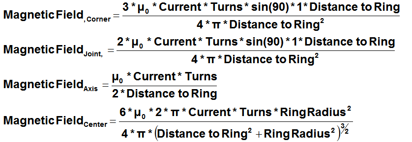


Number
Of Electrons Trapped:
Either gausses law or coulombs law can be used
to find how many electrons are in the center.
The key inputs are the voltage drop (10 kV) and the distance at which it
is measured. There is no indication that
a Langmuir probe was used to measure the voltage drop. The drop must have been estimated. The distance therefore, is taken from where
the deuterium ions form. This spot to
ring center is 0.201 ± 0.017 meters. From
this, coulomb's’ law predicts between 1.5 and 1.2E12 net electrons.
The Sydney paper [35]
models the magnetic field as a superposition of six, single ring fields. The field from a single of current can be
predicted mathematically. This expression
is found in reference [15] a classical physics textbook. It is an equation in polar coordinates (Z,
Rho). This is written out below.

In these equations, K and E are the
complete elliptical integral of the first and second kind. They are difficult to deal with. They arise from ellipses. They are the arch length of an ellipse. They had to be looked up [25]. This math required that Z and rho had to be
greater than zero and below one. This
meant that absolute values were used.
Additionally, this function cannot handle zero. When this occurred, these results were set to
zero.
Trapezoid Approximation In Excel:
An excel model was created. The equations were easy to enter into a
spreadsheet but the elliptical integrals had no function. To compute them, a simple approximation was needed. This was found [25]. The approximation estimated the elliptical
integrals using the trapezoidal rule. This
is done out to four terms. It is valid
to three decimal places. The estimate is
compared to the real values below. The difference
is a problem at high field strengths.
This happens at the joints. There will be a difference between Excel and
MATLAB estimates at the joints.

MATLAB Model Of Single Ring:
A
MATLAB model was also created. The
program can solve the elliptic integrals with the command [K, E] =
ellipke(M). This code gave the field for
a single ring at any X Y and Z coordinates.
From this code a vector field was generated. This is included below for the XY plane around
a single isolated ring. As expected: the
field swirls around the ring of current.
The field generally points from left to right. The strength crests when the particle passes
through ring center. On the right side
the Y fields point away from the axis. I
hope to upload this code online for others to use.
Verifying Excel and MATLAB:
Both codes needed to be verified. Simple math is the best way to do this. The fields are modeled for a particle flying
on axis towards one ring. There are five
methods for calculating this field. The
first is a simple calculator provided by hyper physics [21] and this is plotted
below. The second is Bussards’
estimation of ~1,000 gauss [2] inside the machine. The third is simple estimates from the
“moving the rings” section. The last two
methods are the Excel and MATLAB codes. For
verification: each method should yield similar results.
Each of the five methods are plotted below. The models agree. The simple model plotted is the magnetic
field calculated on axis [21]. One new result
was the MATLAB and Excel codes show a radial field. This a reasonable result. The field generates the swirling vectors
around the rings. This is symmetric
around the axis so it could be in the Y or Z plane. This field causes the electrons to corkscrew
as they approach the rings [34]. Beyond
this, any prediction of electron motion is limited by electron-electron
interactions. 
Energy Density Analysis
If you combine the electric and magnetic fields,
you can make a total “energy density map” for the system. The equation used for this is shown below and
typical numbers are shown for a single ring.
Note that the equation requires magnetic field values in Teslas. The B field used is the average of the radial
and z directed fields.

Part 3: The Complete Magnetic Field
Put the same magnetic
poles together, and they will push apart.
Two north poles are not happy when shoved together. The vector field they make is shown in the
above image. They also have a high
energy density between them. The energy
density goes up when a third north pole is add. The polywell is similar. It is six magnets in a cube. The same pole is pushed together six
times. Intuitively then, we expect the
vector field to fly outwards in all directions.
In general, this is the case. The
only place this is not true is through the rings themselves. The fields are pointed inward through the
rings. In a way, the rings act like six
“doors” to a home. The fields come in
through the doors, and fly outwards everywhere else.
How could such a
system contain electrons? The reason is
the magnetic mirror effect. The
electrons that fly away from the center and are moving into denser fields. The fields get so dense – especially at the
corners – that the electron hits a magnetic mirror and are reflected. Containment inside the polywell may be a
balance between these two physical mechanisms: the fields spraying material
outward in all directions and the magnetic mirror reflecting material back into
device center.
The
Complete Magnetic Field:
To
model all six rings, you need to combine each single ring field together. This is done using superposition. In practice, this means adding the vectors that
are on axis, together. The vectors to
are added when they point in the same directions. They are subtracted when they point in
opposing directions. This is taken from the 2011 Sydney paper [35]. That paper used the model for one ring, six times. Each ring generates two polar fields; one in
the z direction and one in the rho direction.
This makes 12 vectors. So for any
point inside the rings, there are twelve vectors which describe the B
field. Now we need to combine them. Combining means adding them together. Hence, the equations for the B field in the x, y and z directions are groups of these 12 vectors. In practice, the rings had to be numbered. The distances from the rings to the location of interest were either +S or -S depending which ring. Also, a term was also needed to account for the switch from polar to Cartesian coordinates. For example, six polar fields make up the x directed field. These are: four radial fields and two axis fields. It is easier to keep track of which polar field goes with the x direction when you see it. This is drawn out below.

There are several
tricks with working with these equations.
The first is keeping track of which coordinates go with which rings. For the modeling done here the point (0, 0,
0) is at the dead center of the rings. Following
the conventions shown above, the other two vector fields can be described. These are shown below.

Working with these equations is difficult.
The equations are easy to enter into excel and MATLAB; but getting the vectors
to point in the correct directions is challenging. This MATLAB code may be uploaded to the web
for others to push it too perfection. Any
small flaws in the code are a moot point, since any model is not reality. The point of the model is a gain a deep
physical understanding of this machine.
Excel:
Paths to Center
The
above equations tell us the magnetic field at different locations. These were put into excel. From the joint, corner and axis there are three
paths into the center of the rings. The
fields can be modeled as the particle “walks” these paths. This can be used as a check as models become
more complex. We expect the repulsive
force to increase as the particle moves into device center. This is analogous to the fields from two
a-like poles placed close together. At
the dead center, the fields should suddenly drop to zero. This is the null point and it scatters the
electrons.
The
first path of interest is just off axis.
Imagine the particle starting at the cage and moving in to the center. As it moves inward it is buffeted by strong
magnetic and electric fields. Off axis,
there is a strong magnetic field pointing inwards. The particle is swimming along with this
“current.” The strongest field (~250 G) is
inside a single ring. This is pointing
into the center. This field quickly reverses
direction as the particle enters the ring structure. This is similar to the fields of six north
poles facing inwards.
Difference:
On-Axis/Off-Axis
The
magnetic field is slightly different on-axis (0) and just off-axis
(±1E-8). On axis, the vectors solely
points outward, with all other vector set to zero. This is plotted below. The "current" is forever out from
the center. These numbers are consistent
with earlier estimates. Just off-axis the plots change dramatically. This is plotted above. Note the Y and Z fields in red and
green. These change from zero to the S
shaped curves. They are consistent with
the radial fields for a single ring. They
generate swirling field lines around the rings. These curves are
symmetric. Any downward tug is equally offset
by an upward pull. Outside the rings these
point towards the axis and, on the inside they point away from the axis.
More
Paths In To Center:
This
path can be compared to two others.
These are: a path from the corner into center and the joint into center. The joint is where the rings are connected. The magnetic field is the densest here. Assume a particle passes from the cage,
through the joint into the center. This
path is about three quarters of a meter long.
All the fields along it are planar.
The particle gets pushed left or right - but not up or down. The field points away from the center. The particle is “swimming upstream” as it
moves into the rings. The field peaks at
~1,800 gauss directly between the rings.
Note that this is lower than the field (1,300 gauss) calculated in
“moving the rings” section above. The
planer fields are symmetric - identical in strength, but opposing in direction
Another important path is from the corner of the
cage into the center. This is the path
the deuterium gas travels. The path is
nearly a meter long. It starts from the
cage corner and travels between three rings, into the center. These fields point outward from the
center. The particle moves “upstream” as
it head towards device center. The field
peaks at about ~1,100 gauss when the rings are closest together. These three paths are compared below.
These plots can be checked against published
literature. Figure three from [35] qualitatively
agrees with these plots. The curves of
the field represent a “magnetic cup.” It
appears the easiest entrance to this field is along the axis. This is through the rings where the field
lines can point inward. As the particle
moves inward the fields point outward and this becomes stronger as the particle
reaches machine center. At the center,
the fields do drop to zero. This is the
null point - and it is an important feature of the machines’ geometry.
MATLAB
Model:
From
Excel, these equations were entered into MATLAB. The equations are easy to encode - but
getting the correct vector field was very difficult. The better part of a month was spent attempting
to get this vector field to align. A magnetic vector field is shown below for
WB6. These fields are consistent with
a-like poles being placed close together.
A “zone of no magnetic field” can be seen running along the X and Y
axis. Particles can enter the ring
structure along these field lines.

Part 4: Rudiments Of Simulation
When actually making a simulation, do not fall victim to
cool options and flashy graphics of a software package. Stay focused on the questions you want to
solve. The best simulations are the
simplest and offer the deepest insights into experimentation.
Bussard would have loved an accurate
computer model. Many do not believe that
computers could handle a full Polywell [30].
I did not. I then heard, that the
2012 copy of the MCNPX software could handle 10^12th particles [37]. That code is a kinetics based software. It is often used for tracking neutrons. This was the evidence that pushed that
modeling was indeed a possibility.
Several models have already been made.
A 1.5 dimensional model was done in the early nineties (dubbed the EXL
code). Since then, models have been made
by: HappyJack, AEO
Iran [4], Indrek, The
Navy Team, Dr. Joel Rogers, hobbyists
and Randy. If the Polywell works, there
will certainly be many more models. The
goal here is not to duplicate the previous work. This post is going to broadly discuss
modeling without focusing on any specific method.
The PIC Method:
One approach is to use is a particle in cell
method. This code originated in the
1960s at the Los Alamos National Labs [6]. If you use it, you owe a debt of gratitude to
Frank Harlow and his team. Below is a
visual homage to franks’ team [7]. 
What is
important about the T3 group was their work was ignored and even criticized
through most of the 1960’s [6]. They
published when nobody else seemed to care - and they were ultimately
vindicated. The particle in cell method
fractures volume into cells and material into particles. It tracks how sample particles move through
these cells.
Particles Needed:What particles will we need for modeling the Polywell? First, assume that the fusion products vanish. This makes sense. Helium at ~10 MeV, has so much energy it cannot be held by any of the reactor fields. Second, the neutrons can be ignored. Ideally, the code would just record when a fusion event occurred. This leaves: deuterium gas, electrons and ions, to be modeled. Each object is summarized below [8, 9, 28, 29]. A simulation will probably use “representative” particle to reduce the amount of material needed to be tracked. The computer may track 1 particle for every 1,000 real particles in an experiment.

Particles Energy:
For this simulation the ions and electrons would be
modeled as having bell curves of energy.
Both bell curves have average energies of 2,500 eV. Rider argues that the rate of energy transfer
from the electrons and ion cloud is so fast; that their energy is the same
[10]. Rider even wrote a new energy
transfer equation to show this [11]. In
the 18 years since, only two papers have cited this work and both were written
by Rider himself.
The 3D Mesh:
Meshing
is the act of breaking the volume into small cells. The key is to simplify as much as you
can. If you want to include the axis,
joint, corner and center the smallest the polywell can be broken into, is 48
parts. What is left - looks like
wedge. The wedge uses planes of symmetry
to duplicate behavior and model the whole machine. It is much simpler to work with. The wedge can be broken down further into
chucks of volume with specific particles energies and physical mechanisms. This is shown below.
Within this space there are several chunks of interest. The first is the electron beam. About 40 amps of electrons were released in
the capacitor discharge [2]. It was
assumed these capacitors were halfway between the rings and cage. The magnetic overtakes the electric field at 15
centimeters before the rings. The
electrons reach the axis of the ring at ~2.8E7 meters per second. As they pass into the green region they being
to experience a repelling field point outward from ring center. This pushes them towards the joints and
corners. A simulation would need to model 2.5E10 net electrons.
The next region is where the deuterium gas is puffed in. About 2.7E+18 of deuterium gas
molecules were puffed in. These start at
0.292 meters from ring center. This is a
colossal number of molecules. This simulation
would model one forty eight of 0.002 percent of this. That is 1E12 of uncharged gas molecules and
two ions for each ionization event. The
gas enters at room temperature (0.02 eV).
When it reaches the corner of the rings it exchanges energy with the
electrons and ionizes. These ions fly
into ring center. If they hit, they may
fuse. Only 800,000 deuterium ions
actually fuse over the 0.0004 seconds of the experiment.
Electron
to Ion Ratio:
Researchers
use dimensionless ratios to reduce number of simulations needed. Using typical electron and ions numbers one
can estimate the ion to electron ratio.
This number needs to be below one to maintain they voltage drop. There is strong indication that this ratio
should be very low (0.001 or lower).
Meshing
With Courant Numbers
The courant number [38] is used to properly mesh
any simulation. The number relates the
speed of the particle, the mesh size and the time step. This is shown below. The number should be on the order of one for
all regions of the simulation. The
number of cells and the time step is worked out for typical particle
speeds. These numbers will likely
change, but the mesh can be planned using this approach. Typical numbers are shown below.

Ideas For Future Work:
There is plenty of work to be
done. It is the hope of this blog that
the US government funds this research accordant with its potential. If they fail to do this, other nations may
rapidly catch up. Here are some ideas
for future questions.
1. Magnetic reconnection at the cusps. In
certain plasma settings magnetic field lines reconnect [39]. Are there any configurations in Polywells,
where this exists?

2. Ratio: magnetic mirrors verses rejection. The
field lines point outward everywhere except through the rings. Particles follow these fields into the cusps
and corners. They enter a dense vector
field. The field gets so dense the
particles hits a magnetic mirror and are reflected. Is there a dimensionless ratio for this?

3. X-ray radiation with probabilities. We can
model the ion and electrons clouds as having densities of 1E19 and have a bell
curve of energy centered at 2,500 eV. With
this information, the coulomb logarithm and the Debye length [40] one may
estimate the average distance between electrons or ions. From this, are we able to predict the amount,
rate and type of X-rays coming off the cloud?

4. Reactor design: avoid arching. If you had been
at the WB6 test, the main thing you would have seen was a burst of lightening
from inside the machine. This was
arching. It is a problem. Bussard raised this issue in his Google
presentation. Any experimental system
needs to avoid this. Can reactors be
designed to avoid this problem?
5. Estimating the mirror ratio. Thomas Dolan reviewed the magnetic
mirror ratio in the nineties. What ratio
did Rider use when he assessed the Polywell?
What was the actual mirror ratio in WB6?
Do these agree?
6. Fusor modes of operation. George Miley has shown that fusors
have modes of operation. He has
published work on the subject. Do
Polywells show similar modes of operations under similar conditions?
7. Energy transfer. Lyman Spitzer wrote “physics of
fully ionized gases” the bible on low density plasmas. In it, there is an equation to model energy
transfer for ions entering an electron cloud.
Riders’ 1995 papers similar equations to argue against the
Polywell. Can these equations be applied
to WB6?
8. Plasma instabilities. Marshall Rosenbluth – the pope of
plasma physics – worked out a slew of plasma instabilities for almost any
plasma structure. Which ones apply to
the polywell? Is there a way to
qualitatively compare these competing instabilities with other physical
mechanisms?
9. Ratio: magnetic verses electric fields. Can sets
of experiments be simplified by combining the electric and magnetic field
strength into one dimensionless number?
There may be a way to express this mathematically. Simulations are ideal for exploring the
impact of this number – as the magnetic and electric fields can be changed
quickly.

Conclusion:
The Polywell Blog has pushed the
boundaries of knowledge. If you think
this work is stellar, that’s because it is.
This was done by an A player.
Several times, this blog has gotten ahead of published literature – only
to have concepts printed later. The
Polywell represents frontier technology, new science and promising
potential. It is a pleasure to work
on. It has also been fun explaining
these complex issues in simple language.
Work cannot continue without funding.
Interested parties can contact ThePolywellGuy@gmail.com
for more information. - Bussard, Robert.
"Dear Sir Philip." Letter to Sir Philip. Jan. 2006. MS.
http://forums.randi.org/showthread.php?t=58665#27, n.p.
- Bussard, Robert
W. "The Advent of Clean Nuclear Fusion: Superperformance Space Power
and Propulsion." 57th International Astronautical Congress (2006).
Web.
3. "Ephi - the Simple Physics Simulator." www.mare.ee.
Indrek Mandre, 2007. Web. 08 Apr. 2012.
.
4.
Kazemyzade,
F., H. Mahdipoor, A. Bagheri, S. Khademzade, E. Hajiebrahimi, Z. Gheisari, A.
Sadighzadeh, and V. Damideh. "Dependence of Potential Well Depth on the
Magnetic Field Intensity in a Polywell Reactor." Journal of Fusion
Energy (2011). Web.
- Rogers, Joel G. "A “Polywell” P+11B
Power Reactor.". Web.
- Spalding, Brian.
"New Science: The Development of Computational Fluid Dynamics at Los
Alamos National Laboratory." YouTube. YouTube, 11 May 2010.
Web. 15 Nov. 2012.
- Fromm, Jacob.
"Numerical Solution of the Problem of Vortex Street
Development." Physics of Fluids 6.975 (1963): 975-82. Print.
- Pauling, Linus. College
Chemistry. San Francisco: Freeman, 1964: 57, 4-5
- Nave, R.
"Atomic Radii." Ionization Energy. Georgia State
University, n.d. Web. 15 Nov. 2012.
- Rider, Todd H.
"A General Critique of Inertial-electrostatic Confinement Fusion
Systems." Physics of Plasmas 6.2 (1995): 1853-872. Print.
- Rider, Todd H.,
and Peter J. Catto. "Modification of Classical Spitzer Ion–electron
Energy Transfer Rate for Large Ratios of Ion to Electron
Temperatures." Physics of Plasmas 2.6 (1995): 1873. Print.
- Spitzer, Lyman. Physics
of Fully Ionized Gases. New York: Interscience, 1962. Print.
- "Electronvolt."
Wikipedia. Wikimedia Foundation, 11 Dec. 2012. Web. 15 Nov. 2012.
- Should Google Go Nuclear? Clean, Cheap, Nuclear Power.
Perf. Dr. Robert Bussard. Google Tech Talks. YouTube, 9 Nov. 2206. Web. 15
Sept. 2010. http://video.google.com/videoplay?docid=1996321846673788606#.
- Jackson, John
David. Classical Electrodynamics. 2nd ed. N.p.: Jones &
Bartlett, n.d. Print.
- Duncan, Mark,
and Robert Bussard. Should Google Go Nuclear? (Summary). N.d. MS. Should
Google Go Nuclear? Www.askmar.com. Mark Duncan, 24 Dec. 2008. Web. 4 Feb.
2013.
- "More
Powerful Electro Magnet: Thicker Wire or More Turns?" Yahoo!
Canada Answers -. Yahoo! Canada, 2011. Web. 02 Jan. 2013.
- Chris.
"Talk-Polywell.org :: View Topic - The Brillouin Limit." The
Brillouin Limit. Talk Polywell, 14 Dec. 2008. Web. 02 Jan. 2013.
- Wesson,
J: "Tokamaks", 3rd edition page 115, Oxford University Press,
2004
- Rider, Todd H.
"A General Critique of Inertial-electrostatic Confinement Fusion
Systems." Physics of Plasmas
6.2 (1995): 1853-872. Print.
- Nave, R.
"Magnetic Field of Current Loop." Magnetic Field of a Current
Loop. Georgia State University, n.d. Web. 02 Jan. 2013.
- "Coulomb
Logarithm." QED RSS. Princeton University, 6 June 2006. Web.
02 Jan. 2013. http://qed.princeton.edu/main/PlasmaWiki/Coulomb_logarithm
- Huba, J.D.
"2009 NRL PLASMA FORMULARY." Plasma Physics Division. Naval
Research Laboratory, 2009. Print.
- "Deuterium
Gas Sold by the Liter." Advanced Specialty Gases. Advanced
Specialty Gases Inc, 2009. Web. 02 Jan. 2013.
http://www.advancedspecialtygases.com/Deuterium.htm
- Luke, Yudell L.
"Approximations for Elliptic Integrals." Mathematics of
Computation 22.103 (1968): 627. Print.
- "Summary
Tables of Calculated and Experimental Parameters for Diatomic, Triatomic,
Organic, Silicon, Boron, Alumminum and Organometallic Molecules." Black
Light Power. Http://www.blacklightpower.com/, 18 May 2012. Web. 04
Jan. 2013.
- "Deuterium."
99.96 Atom % D. N.p., n.d. Web. Sigma-Aldrich Inc. 12 Dec. 2012.
- Yoon, Jung-Sik,
Young-Woo Kim, Deuk-Chul Kwon, Mi-Young Song, Won-Seok Chang, Chang-Geun
Kim, Vijay Kumar, and BongJu Lee. "Electron-impact Cross Sections for
Deuterated Hydrogen and Deuterium Molecules." Reports on Progress
in Physics 73.11 (2010): 116401. Print.
- Elert, Glenn,
Michael P, and Judy Dong. "Diameter of an Atom." Diameter of an
Atom. The Physics Factbook, 1996. Web. 04 Nov. 2012.
- Ligon, Thomas.
"The Polywell - Interview With Thomas Ligon (Normal).wmv."
YouTube. YouTube, 28 Jan. 2013. Web. 04 Feb. 2013.
- Tibbets, Dan.
"Talk-Polywell.org :: View Topic - Magrid Configuration
Brainstorming." Talk-Polywell.org. Discussion on the Number of
Ampturns, 15 Nov. 2012. Web. 15 Nov. 2012.
- "BatteryMart:
Purchase RV Batteries." www.BatteryMart.com. Battery Mart Inc., 2013.
Web. 25 Jan. 2013.
- "American
Wire Gauge." Wikipedia. Wikimedia Foundation, 28 Jan. 2013.
Web. 04 Feb. 2013.
- McNamara, David,
and Alan Middleton. "The Vector Cross Product - A JAVA Interactive
Tutorial." Vector Cross Product. Syracuse University Physics
Department, 20 Mar. 1996. Web. 12 Jan. 2012.
- Carr, Matthew,
and David Gummersall. "Low Beta Confinement in a Polywell Modeled
with Conventional Point Cusp Theories." Physics of Plasmas 18.112501
(2011): n. page. Print
- "The Debate
about Dwindling Innovation." The Economist. The Economist
Newspaper, 22 Jan. 2013. Web. 04 Feb. 2013.
- Pelowitz, Denise
B. MCNPX User’s Manual. Apr. 2008. Version 2.6.0. Los Alamos National
Labs, Los Alamos
- "Courant–Friedrichs–Lewy
Condition." Wikipedia. Wikimedia Foundation, 27 Jan. 2013. Web. 06
Feb. 2013.
- "Magnetic
Reconnection." Wikipedia. Wikimedia Foundation, 27 Jan. 2013. Web. 06
Feb. 2013.
- "Debye
Length." Wikipedia. Wikimedia Foundation, 02 June 2013. Web. 06 Feb.
2013.


Hello World!
ReplyDeleteWant your OWN copy of the MATLAB code that was used in this post? Download free copies at:
https://github.com/ThePolywellGuy
Polywell Posts, Sketch up models, Matlab code! All available for free download!
Hi, thanks for the Polywell Blog forcus on simulations. I have researched several plasma fusion models and have some items that might be of use to you. Additionally, I would be willing to integrate these with your models or just deliver them.
Delete1. Fast and accurate Elliptic Integrals (all types, in Excel/VBA, Object Pascal and C., tested! References: BC Carlson: http://dlmf.nist.gov/19#PT3, Asymptopic approximations for symmetric elliptic integrals" http://127.0.0.1:4664/redir?url=http%3A%2F%2Farxiv%2Eorg%2Fabs%2Fmath%2F9310223v1&src=1&schema=2&s=3qJ3xCtXEfF1iiWkH3H5Ts_q7bI.http://apps.nrbook.com/empanel/index.html#pg=309 (but it has an coefficient error which I fixed),"
3. I designed these to to calculate the 3d magnetostatic (or electrostatic) ring configuration fields using your parameters.
2. I have A slow and crude Excel 'perfect' particle confinement inside a 'porous holey' sphere.
I saw non-symmetric compressed cloud circulating about the center.
Also observed the critical dependence of confinement on the energy of the particles and the 'ramping' of confinement voltage.
I Plan to rewrite to C++/Pascal to check.
3. I used a simple 3d FDTD model to calc both static and dynamic EM configuration. I lost the original working model when my computer fried, and I am now rewriting and testing. Missing Planned features: complex PML, spherical modelling and symmetry, geometry specification.
4. I am looking for a decent Vlasov-Darwin plasma model to try with PIC, but I can't figure the math out yet. Am focussing on 'cold' plasmas (initial room temp) to evaluate various confinement geometries as plasma temp and density increase.
5. I purchased a basic high vacuum, two stage system and HV power supply, but have not assembled it. To test the results of the models, since I could not locate any extensive data sets from the various 'fusor' (IEC,etc) groups.
6. I Also have Wolfram Mathematica available as another tool and am working on a FDTD model to simplify the programming required to evaluate the mathematical models.
To my knowledge Rider's critiques have not been addressed by the IEC/Polywell community.
Jim Hargis
8093 S Oneida Ct
Centennial, CO 80112
303-220-0253
jimhargis@comcast.net
Jim!
DeleteYou are the first person to comment in a couple of months. I have a couple of comments and questions.
First - elliptic integrals. The model in "taking a stab at simulation" relied on the first elliptic integral. I solved this in MATLAB with a simple command - but to do an excel model I needed to use an approximation. I got the approximation from this paper. The integral went into a nasty equation which predicted the x, y and z magnetic field inside the Polywell. That set of equations was pulled from Khachan's 2011 paper.
Magnetostatics is a great place to start. If you can do three dimensions you will be ahead of both me and the khackan team. Their latest paper, only did a two dimension simulation. I am working on a review of that paper, right now. Personally, I do not think we need to go three dimensions yet, we can still learn allot more from a two dimensional model. I would love to see a simple Java applet which lets people fuddle with the Polywell parameters to see what kind of behavior pops out. I have described this on Talk-Polywell, but the idea needs development.
Ultimately, I think what we need to do is pair simulations with dimensional analysis. There are many dimensionless numbers in plasma physics and the Polywell has got to have several which affect it. It is also likely that the machine has modes of operation. A good starting point is the fusor, which we know has at least 3 modes of operation - Halo mode, Star Mode and Converged Core mode. Simulations allow us the flexibility to model Polywells that we could never build, and eliminate vast chunks of operating space before we ever build a machine. I would not be surprised if the Navy team has gone down this path already - but unfortunately they are not publishing.
In doing any code, the trickiest part is getting realistic results. You have to get the code to duplicate a real world test. I have wasted a year or so, working with code which I thought was meaningful, but was actually flawed. That is why in "taking a stab" I used four methods to check my results: Bussard's 2006 paper, simple Biot-Savart math, Excel and finally, MATLAB. I am confident in my code - and I encourage anyone to rip it apart. I encourage you to use to benchmark your stuff.
You are using a finite difference model, right? You have the model encoded in some software, right? What is the program that you are running your code in? Certainly excel would be limited - I doubt it would be able to tell you that there is a non-symmetric cloud in the center. I use excel to test simple calculations, to make sure that MATLAB is running correctly. Whenever there is a discrepancy, it leads me to some mistake that needs correcting. It took me about 8 months (off and on) to get excel, Matlab and simple equations to agree.
Also, I am not an expert on finite difference models. Many of the Polywell simulations done by Joel Rogers, Joe Khackan and the Bussard/Krall team were all Particle-in-Cell models. Bussard described a "1.5 dimensional Vlasov-Darwin model" in the early 90's. So, I have heard the term before, but I do not know much about the model, maybe you can explain it to me. Part of what I am so proud of about "The Polywell Blog" is that it explains things in clear language. The easier the posts are for you to read, the longer I took in writing them.
ReplyDeleteBack in March, I was trying to model particle motion. I was using newtons equations of motion to map how the particle moves. Indrek Mare had already looked at this problem and determined modeling it like this would not work. The reason had to do with vectors that were not aligned. Overtime this led to an error between the modeled and real motions which would grow unreasonable. The solution was to use the Runge-Kutta method. I encoded this into Excel and MATLAB, but ultimately had to put the problem on the shelf. I may come back to it. I gave some of the details in this Talk Polywell post.
I think there is enough theory work to go around. This includes tackling Riders works. I explained Rider's 1995 paper here. It took me 8 months to write that review and it is not perfect. I have not had time to work on his thesis. I think the polywell is so complex that it is hard to believe that any one person could fully describe it. I include myself in that. I am humbled by the amount of knowledge needed to understand this machine. So, when a theortican claims he has it figured out, it is hard to believe he didn’t miss something. We should just build it and find out.
Lastly - This stuff is really hard. Nobody knows if it is going to work or fail. It may fail, we do not know. Because it is so complex, my stance has always been to be open about everything. The goal is to make the idea – its’ strengths and weaknesses available to anyone. Hopefully we can build enough interest to get research really moving.
This comment has been removed by a blog administrator.
ReplyDelete